This how-to is for beginners in R. For the next step, try exploring the online book R for Data Science by Garrett Grolemund and Hadley Wickham
What is R?
R is a programming language used for statistical analysis. Think of it like a much more powerful version of Excel, with all of the nice user-interface stripped away. Instead of putting numbers into cells, we create objects. Objects can be individual cells, a collection of cells, an entire column, an entire row, and entire sheet, or an entire Excel workbook. We combine and manipulate objects for our data analysis.
Excel is a program with a user-interface. R is a language for raw computing. Both can accomplish similar tasks, but R is much more versatile, stronger, and free. This how-to was created in R! We won’t unlock the true potential of R here, but this should help you get started.
How do I download R?
Remember, R is a language. For you to use R on your computer, you first need to download the language. Downloading the language is equivalent to teaching your computer how to speak R. Lucky for you, your computer can learn R much faster than you can learn Spanish. Teach your computer how to speak R here:
https://mirror.las.iastate.edu/CRAN/
Once you have downloaded the language, you should make it easier to communicate with your computer. Your computer now knows R, but you still don’t. If you want to communicate with your computer, but still have it do things in R, you should download a studio environment. The studio is a user interface that will allow you to use R, while keeping track of all your objects visually. Your computer has no eyes, but you do. A studio is for our humble human benefit. Download RStudio here:
https://rstudio.com/products/rstudio/download/
How do I start R for the first time?
Once you have downloaded R and RStudio, you are ready to open R for the first time. Let’s start by opening R.
On your computer, you will have two new R programs:

First, open R (the program simply called “R”). You will see:
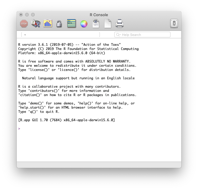
This is the console: a window where you type commands, and the computer responds. Try typing the following into the console, then hit enter:
2 + 2
As you can see, R will recognize that you are asking what “2+2” equals, and will provide the output: 4. Try a few other simple math problems. Now close the R program and don’t ever open it again.
The console is great, but as you progress, you’ll want to save some of
your commands so you don’t have to re-type them every time. A list of
commands is called a script. Sometimes you’ll want to produce a
table or a graph or a regression, but not have a new window pop up with
the output. Sometimes you may want to glance at the contents of your
current working directory and see all the datasets you have available,
or the list of variables you have created. In R, these objects are
invisible until you explicitly ask R to show you. For that reason, we
are going to use RStudio, where all of the above is visible at once.
Now, open the RStudio program. You should see the following (without
the red numbers):
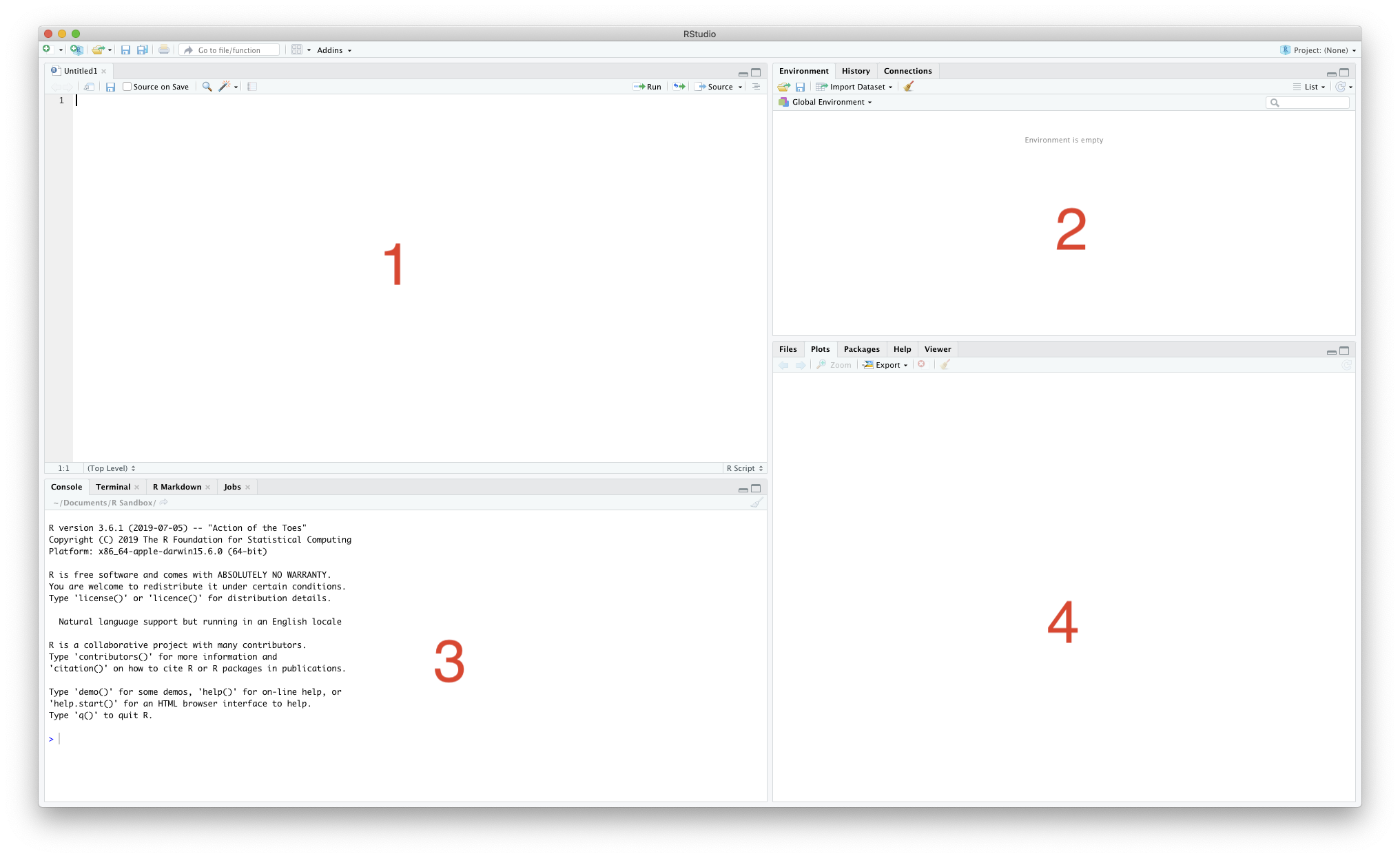
The RStudio environment is split into four panes, labelled in the image above. Let’s explore each:
-
1: This is the script editor. If you want to write a series of commands, and you want those commands to run immediately after each other automatically, you’ll need to write a script. When we begin writing code, we will use this pane. Scripts are the cornerstone of replicating your work, and replication is paramount in good research and data science.
-
2: This is where you will be able to see all of the variables, data frames (the R word for data sets), lists, and any other objects that you have created. If you create it, it will show up here.
-
3: This is the console! It is the same thing that you saw when you opened the basic R program. Here, we just keep it in a single pane. Think of it as the actual place where you and your computer talk in R. You write a script, but then it is run in the console. You can also write commands directly in the console. You’ll also see some results in the console, though plots are shown in pane 4.
-
4: This is where you will see any plots you create, and where you’ll find help files. You can also look at the contents of your working directory and the packages that you currently have downloaded.
Basic R Syntax
Open RStudio. You should see the 4-pane setup from above. To establish good habits early, we are going to work in the script editor (pane 1). Working in the console gives you immediate results, but saving the history of your commands in a single document –a script– is very useful if you ever need to “de-bug” your commands. Because we are working in the script editor, once you type a line of code (a command) and hit enter, nothing happens. In script mode, your computer is ignoring you until you are done writing commands. To wake up your computer and tell it to run the commands, you need to highlight the commands you want to evaluate, and hit “Run”. You can either click the button at the top right corner of pane 1 (where it says “Run”), or highlight the code you want to run and hit “⌘ + enter” (or “Ctrl + enter” on a PC). If you want to run the entire script, hit “⌥ ⌘R”.
- Do some math: One of the most basic functionalities of R is the ability to perform simple math. Try typing (not just copy+paste) the following commands in the script editor, then ask R to run the script and evaluate all the commands.
2+2
2-3
3/9
4^5
6**2
What happens? You should see the results in the console. Your input (commands) have a “>” symbol in front of them, and the output has a “[1]”. These are just indications for when you are talking vs when the computer is talking. The code you just ran can be written as a story:
“What is 2 plus 2?” you asked.
“4” the computer replied.
“What is 2 minus 3?” you asked.
“-1” the computer replied.
…and so on: it is not an elegant conversation, but it is a conversation nonetheless.
- Create an object: There are many types of objects we can create in R, so I’m only going to focus on the most common: variables, scalars, and data frames. We’ll start with creating a scalar. Remember that a scalar is just a number, but sometimes we want to save a particular number to reference or use over and over again. For example, suppose you want to derive β̂1 in a basic univariate linear model. For a variable x, you’ll need to know x̄: the sample mean. Suppose that mean is 4. We can create a scalar called “xmean” and make it take the value of 4:
xmean <- 4
The <- symbol is the command for assignment. We can interpret the
above command as: “Assign the value of 4 to the word ‘xmean’”. Now, we
can use the word “xmean” and your computer will know you mean 4:
xmean <- 4
xmean*3

## [1] 12
Perhaps a bit weirdly, the <- symbol can also work as ->. So the
above chuck of code can also be run as:
4 -> xmean
xmean*3

## [1] 12
The proper etiquette is to write assignments using <- and not ->.
The object should go first, then the assignment arrow, then the value
you are assigning to the object. The order doesn’t technically matter; R
will understand either direction of logic/arrow. To make things
consistent in case you want to share your commands or need help, it is
important to stick to established rules and use <-.
Starting a Script
R has thousands of user-written packages. The “base-R” that you downloaded is the basic program, and while it can do a lot, smart people from around the world have written special programs to teach R how to do more. In fact, you may find that much of what you do requires an additional package beyond the base version of R you have right now.
To start a script you should do the following:
- Comment and describe the purpose of your script. When you put a
#on any line in a script, everything after the#is considered a comment, and R will ignore it:
# This is an R script to add 2 and 2
# Written by: Jean-Luc Picard
2+2
- Install and load packages that will appear anywhere in the
script. Packages are called libraries, which makes a lot of sense.
Every time you launch R, it will start exactly the same way you
started it the first time, with the same set of knowledge. If you
want it to do some cool stuff found in another package, you have to
tell R to go to a specific library to learn the skill, then remind
it every time that skill is found in some specific library. You need
to first tell R to
install.packages("<package name>"), thenlibrary("<package name>"). You only need to install a package once ever. You need to load the library every time you want to use it. Again, etiquette dictates that we put all libraries for a script at the top:
# This is an R script to add 2 and 2
# Written by: Jean-Luc Picard
# install.packages("ggplot2")
library(ggplot2)
If you run the above code, you should get an error. You tried to load
the library without first installing it. The
install.packages("ggplot2") command didn’t work because it was
commented out. Remove the # and try again.
An important note: many libraries come with their own sample data, in addition to a suite of commands.
- Set your working directory. You need to tell R what folder to work in. You computer has many folders and sub-folders where you can put stuff, so you need to give your R session a home. When you set the working directory, all of the files in that directory (folder) are viewable by R without having to specify a file path:
# This is an R script to add 2 and 2
# Written by: Jean-Luc Picard
# install.packages("ggplot2")
library(ggplot2)
setwd("<your local path>")
Import your data
Sometimes the packages you load have built-in data for you to play
around with. For example, the ggplot2 package has a built-in dataset
called economics. Tell R you want to load this data with the command
data('economics') after you have loaded the ggplot2 package. Then,
we can assign that dataset to a new name like 'econ' for brevity
# This is an R script to add 2 and 2
# Written by: Jean-Luc Picard
# install.packages("ggplot2")
library(ggplot2)
setwd("<your local path>")

data('economics')
econ <- economics
Most of the time, however, you’ll need to import your data from other
sources. Three common import files are .CSV, .XLS (.XLSX), and .DTA. For
the following, assume that your raw data file is called “RawData”. We
will import “RawData”, and assign it to the object data, which is a
dataframe.
- Import from a CSV file:
setwd("<your local path>")
data <- read.csv("./RawData.csv")
- Import from an XLS or XLSX file:
install.packages("readxl")
library(readxl)
data <- read_excel("./RawData.xlsx")
- Import from a Stata (DTA) file:
install.packages("haven")
library(haven)
data <- read_dta("./RawData.dta")
Notice that importing CSV files does not require any additional package, but importing Excel or Stata files does require additional packages.
Clean your data
After importing your data, you may need to clean it. That is, make sure the variables are in the right format for whatever economic model you want to estimate. The process of cleaning, or wrangling your data is unfortunately sometimes complicated and a bit of an art form. This short tutorial does not cover data cleaning.
Estimate your model
Once you have imported and cleaned your data, you are ready to estimate
a model. We will start with one of the first regressions we ran in AGEC
317:
$$mpg_i = \beta_0 + \beta_1weight_i + \beta_2cyl_i + \beta_3 disp_i + \varepsilon_i$$
where $mpg_1$ is the fuel efficiency of car i in
miles-per-gallon, $weight_i$ is the weight in
thousands of pounds, $cyl_i$ is the number of cylinders
in the engine, and $disp_i$ is the engine size in
cubic inches. We are interested in the partial effects of weight, number
of cylinders, and engine size on a vehicle’s fuel efficiency.
So how would we perform a linear regression? In Excel, we make several
cumbersome clicks and it takes a while. In R, we use the command lm(),
short for “linear model”. There are two arguments for the linear model
function: the formula of the regression, and the dataset we are using.
For the lm() regression formula, write the dependent variable, then a
~, then all of the independent variables separated with a + sign.
After writing the regression formula, put a comma, then
data=<name of dataset>. For example, try running the following script
(note that you need to install and load the package dplyr):
# This is an R script to perform a linear regression
# Written by: Jean-Luc Picard
# install.packages("ggplot2")
library(dplyr)
setwd("/Users/michaelblack/Documents")

data('mtcars')
cars <- mtcars
lm(mpg ~ wt + cyl + disp, data = cars)

##
## Call:
## lm(formula = mpg ~ wt + cyl + disp, data = cars)
##
## Coefficients:
## (Intercept)           wt          cyl         disp
##   41.107678    -3.635677    -1.784944     0.007473
You should see the same results. But those are just the coefficient
estimates! We don’t know whether the coefficients are statistically
significant or not, and we don’t know anything about the model fit. When
R performs a linear regression using lm(), it actually generates a lot
of information, but doesn’t automatically report it to you. What we want
to do is assign all of the regression information to an object, and then
summarise the object!
# This is an R script to perform a linear regression
# Written by: Jean-Luc Picard
# install.packages("ggplot2")
library(dplyr)
setwd("/Users/michaelblack/Documents")

data('mtcars')
cars <- mtcars
regression <- lm(mpg ~ wt + cyl + disp, data = cars)
summary(regression)

##
## Call:
## lm(formula = mpg ~ wt + cyl + disp, data = cars)
##
## Residuals:
##     Min      1Q  Median      3Q     Max
## -4.4035 -1.4028 -0.4955  1.3387  6.0722
##
## Coefficients:
##              Estimate Std. Error t value Pr(>|t|)
## (Intercept) 41.107678   2.842426  14.462 1.62e-14 ***
## wt          -3.635677   1.040138  -3.495  0.00160 **
## cyl         -1.784944   0.607110  -2.940  0.00651 **
## disp         0.007473   0.011845   0.631  0.53322
## ---
## Signif. codes:  0 '***' 0.001 '**' 0.01 '*' 0.05 '.' 0.1 ' ' 1
##
## Residual standard error: 2.595 on 28 degrees of freedom
## Multiple R-squared:  0.8326, Adjusted R-squared:  0.8147
## F-statistic: 46.42 on 3 and 28 DF,  p-value: 5.399e-11
There you go! We see the model fit information at the bottom of the output, and information on the standard errors and p-value of the individual coefficients. The last step is to know how to generate new variables like squared terms and logged variables.
There are lots of ways to create new variables. A popular approach is to
use the dplyr command: mutate(). That, however, is a lesson for
another day. For now, we are going to use a straightforward approach.
First, note that to reference a column within a dataset, you write the
name of the dataset, then a $, then the name of the column. So if you
want R to look at the mpg column of the cars dataset, write
mpg$cars. If you want to create a new variable, just assign that new
variable to a column that does not yet exist, and you will force it into
existence! Take a look at the following script:
# This is an R script to perform a linear regression
# Written by: Jean-Luc Picard
# install.packages("ggplot2")
library(dplyr)
setwd("/Users/michaelblack/Documents")

data('mtcars')
cars <- mtcars
cars$wt2 <- cars$wt^2
cars$lndisp <- log(cars$disp)
regression <- lm(mpg ~ wt + wt2 +cyl + disp + lndisp, data = cars)
summary(regression)
You just:
-
Imported data
-
Created two new variables
-
Estimated a non linear economic model
-
Presented the regression results
And all without clicking! Your code is transparent, and anyone with your code can replicate your results and see exactly what you did.